In this tutorial, we will learn how to recognize handwritten digit using a simple Multi-Layer Perceptron (MLP) in Keras. We will also learn how to build a near state-of-the-art deep neural network model using Python and Keras. A quick Google search about this dataset will give you tons of information - MNIST.
Update: As Python2 faces end of life, the below code only supports Python3.
This tutorial is intended for beginners exploring how to implement a neural network using Keras. We will strictly focus towards the implementation of a neural network without concentrating too much on the theory part. To learn more Deep Learning theory, please visit this awesome website.
Note: Before implementing anything in code, we need to setup our environment to do Deep Learning. Make sure you use the below links to do that and then come here.
1
2
3
4
5
6
7
* What is MNIST dataset?
* How to load and pre-process MNIST dataset in Keras?
* How to use one-hot encoding in Keras?
* How to create a multi-layer perceptron in Keras?
* How to perform Deep Learning on MNIST dataset using Keras?
* How to save history of model and visualize metrics using Keras and matplotlib?
* How to recognize digits in real-images by segmenting each digit and then classifying it?
Dependencies
You will need the following software packages and libraries to follow this tutorial.
- Python
- NumPy
- Matplotlib
- Theano or TensorFlow
- Keras
Pipeline
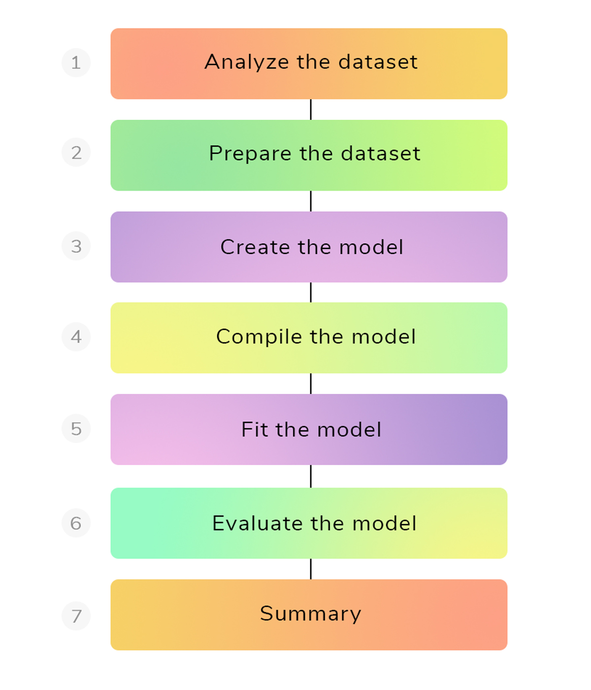
Any deep learning implementation in Keras follows the below pipeline. It is highly recommended that you go through this first before writing any code so that you get a clear sense of what you are going to achieve through Deep Learning.
Dataset summary
- MNIST - Mixed National Institute of Standards and Technology database.
- Created by - Yaan LeCun, Corinna Cortes, Christopher Burges.
- Image size - 28 x 28 pixel square (784 pixels in total).
- Training images - 60,000
- Testing images - 10,000
- Top error rate - 0.21 (achieved by CNN)
- Dataset size in Keras - 14.6 MB
Note: To look at state-of-the-art accuracies on standard datasets such as MNIST, CIFAR-10 etc., please visit this excellent website by Rodrigo Benenson.
Organize imports
We will need the following python libraries to build our neural network.
- NumPy - To perform matrix/vector operations as we are working with Images (3D data).
- Matplotlib - To visualize what’s happening with our neural network model.
- Keras - To create the neural network model with neurons, layers and other utilities.
1
2
3
4
5
6
7
8
9
10
11
# organize imports
import numpy as np
import matplotlib.pyplot as plt

from keras.models import Sequential
from keras.layers.core import Dense, Activation, Dropout
from keras.datasets import mnist
from keras.utils import np_utils

# fix a random seed for reproducibility
np.random.seed(9)
Define user inputs
In a neural network, there are some variables/parameters that could be tuned to obtain good results. These variables are indeed user inputs which needs some experience to pick up the right one. Such user-defined inputs are given below -
- nb_epoch - Number of iterations needed for the network to minimize the loss function, so that it learns the weights.
- num_classes - Total number of class labels or classes involved in the classification problem.
- batch_size - Number of images given to the model at a particular instance.
- train_size - Number of training images to train the model.
- test_size - Number of testing images to test the model.
- v_length - Dimension of flattened input image size i.e. if input image size is [28x28], then v_length = 784.
1
2
3
4
5
6
7
# user inputs
nb_epoch = 25
num_classes = 10
batch_size = 128
train_size = 60000
test_size = 10000
v_length = 784
Prepare the dataset
- Loading the MNIST dataset is done simply by calling mnist.load_data() function in Keras. It returns two tuples holding (train data and train label) in one tuple, and (test data and test label) in another tuple.
- If you run this function for the first time, it will download the MNIST dataset to a local folder ~/.keras/datasets/mnist.pkl.gz which is 14.6 MB in size.
- After loading the dataset, we need to make it in a way that our model can understand. It means we need to analyze and pre-process the dataset.
- Reshaping - This is needed because, in Deep Learning, we provide the raw pixel intensities of images as inputs to the neural nets. If you check the shape of original data and label, you see that each image has the dimension of [28x28]. If we flatten it, we will get 28x28=784 pixel intensities. This is achieved by using NumPy’s reshape function.
- Data type - After reshaping, we need to change the pixel intensities to float32 datatype so that we have a uniform representation throughout the solution. As grayscale image pixel intensities are integers in the range [0-255], we can convert them to floating point representations using .astype function provided by NumPy.
- Normalize - Also, we normalize these floating point values in the range (0-1) to improve computational efficiency as well as to follow the standards.
1
2
3
4
5
6
# split the mnist data into train and test
(trainData, trainLabels), (testData, testLabels) = mnist.load_data()
print("[INFO] train data shape: {}".format(trainData.shape))
print("[INFO] test data shape: {}".format(testData.shape))
print("[INFO] train samples: {}".format(trainData.shape[0]))
print("[INFO] test samples: {}".format(testData.shape[0]))
[INFO] test data shape: (10000L, 28L, 28L)
[INFO] train samples: 60000
[INFO] test samples: 10000
1
2
3
4
5
6
7
8
9
10
11
12
# reshape the dataset
trainData = trainData.reshape(train_size, v_length)
testData = testData.reshape(test_size, v_length)
trainData = trainData.astype("float32")
testData = testData.astype("float32")
trainData /= 255
testData /= 255

print("[INFO] train data shape: {}".format(trainData.shape))
print("[INFO] test data shape: {}".format(testData.shape))
print("[INFO] train samples: {}".format(trainData.shape[0]))
print("[INFO] test samples: {}".format(testData.shape[0]))
[INFO] test data shape: (10000L, 784L)
[INFO] train samples: 60000
[INFO] test samples: 10000
One Hot Encoding
The class labels for our neural network to predict are numeric digits ranging from (0-9). As this is a multi-label classification problem, we need to represent these numeric digits into a binary form representation called as one-hot encoding.
It simply means that if we have a digit, say 8, then we form a table of 10 columns (as we have 10 digits), and make all the cells zero, except 8. In Keras, we can easily transform numeric value to one-hot encoded representation using np_utils.to_categorical function, which takes in labels and number of class labels as input.
For better understanding, see the one-hot encoded representation of 5, 8 and 3 below.
| d | b0 | b1 | b2 | b3 | b4 | b5 | b6 | b7 | b8 | b9 |
|---|---|---|---|---|---|---|---|---|---|---|
| 5 | 0 | 0 | 0 | 0 | 0 | 1 | 0 | 0 | 0 | 0 |
| 8 | 0 | 0 | 0 | 0 | 0 | 0 | 0 | 0 | 1 | 0 |
| 3 | 0 | 0 | 0 | 1 | 0 | 0 | 0 | 0 | 0 | 0 |
1
2
3
# convert class vectors to binary class matrices --> one-hot encoding
mTrainLabels = np_utils.to_categorical(trainLabels, num_classes)
mTestLabels = np_utils.to_categorical(testLabels, num_classes)
Create the model
We will use a simple Multi-Layer Perceptron (MLP) as our neural network model with 784 input neurons.
Two hidden layers are used with 512 neurons in hidden layer 1 and 256 neurons in hidden layer 2, followed by a fully connected layer of 10 neurons for taking the probabilities of all the class labels.
ReLU is used as the activation function for hidden layers and softmax is used as the activation function for output layer.
After creating the model, a summary of the model is presented with different parameters involved.
We are still allowed to tune these parameters (called as hyperparameters) based on the model’s performance. In fact, there are algorithms to get the best possible hyper-parameters for our model which could be read here.
1
2
3
4
5
6
7
8
9
10
11
12
13
# create the model
model = Sequential()
model.add(Dense(512, input_shape=(784,)))
model.add(Activation("relu"))
model.add(Dropout(0.2))
model.add(Dense(256))
model.add(Activation("relu"))
model.add(Dropout(0.2))
model.add(Dense(num_classes))
model.add(Activation("softmax"))

# summarize the model
model.summary()
Compile the model
After creating the model, we need to compile the model for optimization and learning. We will use categorical_crossentropy as the loss function (as this is a multi-label classification problem), adam (gradient descent algorithm) as the optimizer and accuracy as our performance metric.
1
2
# compile the model
model.compile(loss="categorical_crossentropy", optimizer="adam", metrics=["accuracy"])
Fit the model
After compiling the model, we need to fit the model with the MNIST dataset. Using model.fit function, we can easily fit the created model. This function requires some arguments that we created above. Train data and train labels goes into 1st and 2nd position, followed by the validation_data/validation_split. Then comes nb_epoch, batch_size and verbose. Verbose is for debugging purposes. To view the history of our model or to analyse how our model gets trained with the dataset, we can use history object provided by Keras.
1
2
# fit the model
history = model.fit(trainData, mTrainLabels, validation_data=(testData, mTestLabels), batch_size=batch_size, nb_epoch=nb_epoch, verbose=2)
Evaluate the model
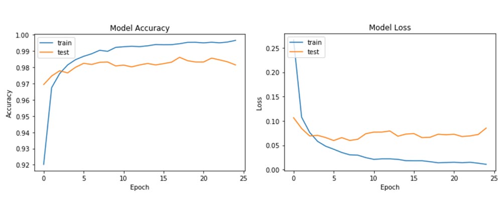
After fitting the model, the model can be evaluated on the unseen test data. Using model.evaluate function in Keras, we can give test data and test labels to the model and make predictions. We can also use matplotlib to visualize how our model reacts at different epochs on both training and testing data.
1
2
3
4
5
6
7
8
9
10
11
12
13
14
15
16
17
18
19
20
21
22
23
24
25
26
27
# print the history keys
print(history.history.keys())

# evaluate the model
scores = model.evaluate(testData, mTestLabels, verbose=0)

# history plot for accuracy
plt.plot(history.history["acc"])
plt.plot(history.history["val_acc"])
plt.title("Model Accuracy")
plt.xlabel("Epoch")
plt.ylabel("Accuracy")
plt.legend(["train", "test"], loc="upper left")
plt.show()

# history plot for accuracy
plt.plot(history.history["loss"])
plt.plot(history.history["val_loss"])
plt.title("Model Loss")
plt.xlabel("Epoch")
plt.ylabel("Loss")
plt.legend(["train", "test"], loc="upper left")
plt.show()

# print the results
print("[INFO] test score - {}".format(scores[0]))
print("[INFO] test accuracy - {}".format(scores[1]))
[INFO] test score - 0.0850750412192
[INFO] test accuracy - 0.9815
Results
As you can see, our simple MLP model with just two hidden layers achieves a test accuracy of 98.15%, which is a great thing to achieve on our first attempt. Normally, training accuracy reaches around 90%, but test accuracy determines how well your model generalizes. So, it is important that you get good test accuracies for your problem.
Complete code
1
2
3
4
5
6
7
8
9
10
11
12
13
14
15
16
17
18
19
20
21
22
23
24
25
26
27
28
29
30
31
32
33
34
35
36
37
38
39
40
41
42
43
44
45
46
47
48
49
50
51
52
53
54
55
56
57
58
59
60
61
62
63
64
65
66
67
68
69
70
71
72
73
74
75
76
77
78
79
80
81
82
83
84
85
86
87
88
89
90
# organize imports
import numpy as np
import matplotlib.pyplot as plt
from keras.models import Sequential
from keras.layers.core import Dense, Activation, Dropout
from keras.datasets import mnist
from keras.utils import np_utils

# fix a random seed for reproducibility
np.random.seed(9)

# user inputs
nb_epoch = 25
num_classes = 10
batch_size = 128
train_size = 60000
test_size = 10000
v_length = 784

# split the mnist data into train and test
(trainData, trainLabels), (testData, testLabels) = mnist.load_data()
print("[INFO] train data shape: {}".format(trainData.shape))
print("[INFO] test data shape: {}".format(testData.shape))
print("[INFO] train samples: {}".format(trainData.shape[0]))
print("[INFO] test samples: {}".format(testData.shape[0]))

# reshape the dataset
trainData = trainData.reshape(train_size, v_length)
testData = testData.reshape(test_size, v_length)
trainData = trainData.astype("float32")
testData = testData.astype("float32")
trainData /= 255
testData /= 255

print("[INFO] train data shape: {}".format(trainData.shape))
print("[INFO] test data shape: {}".format(testData.shape))
print("[INFO] train samples: {}".format(trainData.shape[0]))
print("[INFO] test samples: {}".format(testData.shape[0]))

# convert class vectors to binary class matrices --> one-hot encoding
mTrainLabels = np_utils.to_categorical(trainLabels, num_classes)
mTestLabels = np_utils.to_categorical(testLabels, num_classes)

# create the model
model = Sequential()
model.add(Dense(512, input_shape=(784,)))
model.add(Activation("relu"))
model.add(Dropout(0.2))
model.add(Dense(256))
model.add(Activation("relu"))
model.add(Dropout(0.2))
model.add(Dense(num_classes))
model.add(Activation("softmax"))

# summarize the model
model.summary()

# compile the model
model.compile(loss="categorical_crossentropy", optimizer="adam", metrics=["accuracy"])

# fit the model
history = model.fit(trainData, mTrainLabels, validation_data=(testData, mTestLabels), batch_size=batch_size, nb_epoch=nb_epoch, verbose=2)

# print the history keys
print(history.history.keys())

# evaluate the model
scores = model.evaluate(testData, mTestLabels, verbose=0)

# history plot for accuracy
plt.plot(history.history["acc"])
plt.plot(history.history["val_acc"])
plt.title("Model Accuracy")
plt.xlabel("Epoch")
plt.ylabel("Accuracy")
plt.legend(["train", "test"], loc="upper left")
plt.show()

# history plot for accuracy
plt.plot(history.history["loss"])
plt.plot(history.history["val_loss"])
plt.title("Model Loss")
plt.xlabel("Epoch")
plt.ylabel("Loss")
plt.legend(["train", "test"], loc="upper left")
plt.show()

# print the results
print("[INFO] test score - {}".format(scores[0]))
print("[INFO] test accuracy - {}".format(scores[1]))
Testing the model
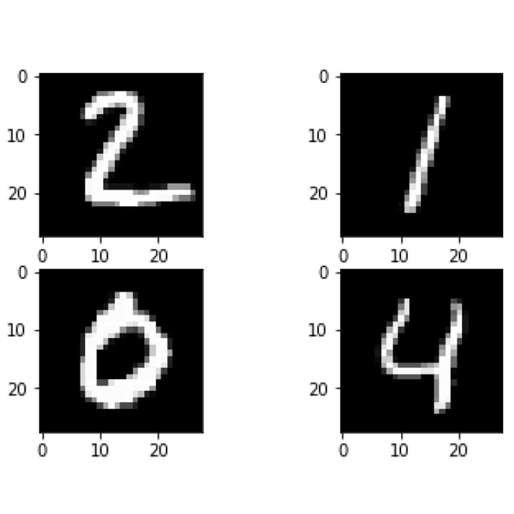
In order to test the model, we can use some images from the testing dataset. These are taken from the testing dataset because these images are unknown to our model, so that we can test our model’s performance easily. We will grab few images from those 10,000 test images and make predictions using model.predict_classes function which takes in the flattened raw pixel intensities of the test image.
1
2
3
4
5
6
7
8
9
10
11
12
13
14
15
16
17
18
19
20
21
22
23
24
25
26
import matplotlib.pyplot as plt

# grab some test images from the test data
test_images = testData[1:5]

# reshape the test images to standard 28x28 format
test_images = test_images.reshape(test_images.shape[0], 28, 28)
print("[INFO] test images shape - {}".format(test_images.shape))

# loop over each of the test images
for i, test_image in enumerate(test_images, start=1):
	# grab a copy of test image for viewing
	org_image = test_image

	# reshape the test image to [1x784] format so that our model understands
	test_image = test_image.reshape(1,784)

	# make prediction on test image using our trained model
	prediction = model.predict_classes(test_image, verbose=0)

	# display the prediction and image
	print("[INFO] I think the digit is - {}".format(prediction[0]))
	plt.subplot(220+i)
	plt.imshow(org_image, cmap=plt.get_cmap('gray'))

plt.show()
[INFO] I think the digit is - 2
[INFO] I think the digit is - 1
[INFO] I think the digit is - 0
[INFO] I think the digit is - 4
Summary
Thus, we have built a simple Multi-Layer Perceptron (MLP) to recognize handwritten digit (using MNIST dataset). Note that we haven’t used Convolutional Neural Networks (CNN) yet. As I told earlier, this tutorial is to make us get started with Deep Learning.
To build a system that is capable of recognizing our own hand-writing, we must take one step further to apply this approach i.e. we need to segment each digit in our hand-written image and then make our model to predict each segmented digit.
In case if you found something useful to add to this article or you found a bug in the code or would like to improve some points mentioned, feel free to write it down in the comments. Hope you found something useful here.